Benchmarking Compression Programs
My main question is: which program should I use for compression?
The answer is not very simple.
It’s rather obvious that it will take longer to compress a bigger file than a smaller one. But will that be twice longer for a twice bigger file?
Are you able to sacrifice compressing a file for another hour just to make it a little bit smaller?
What about decompressing time?
Is it true that decompressing time depends on the compression level?
Data Respository
All the files, including this notebook, can be found at https://github.com/szymonlipinski/compression_benchmark
Testing Procedure
For generating the data I used the generate_data.py script.
Programs
I have tested five compression programs:
- zip
- gzip
- bz2
- lzma
- xz
Compression Levels
Each of them can be run with a compression level argument which can have values from 1 to 9.
File Sizes
As this analysis is a side effect of another project, where I analyse chess games downloaded from lichess, I used a lichess file. Each of the files contain only alphanumeric characters with chess PGN notation.
You can find the lichess files at https://database.lichess.org/.
I used files with different sizes:
- 1kB
- 10kB
- 100kB
- 1MB
- 10MB
- 100MB
- 1GB
Machine Spec
- CPU: Intel(R) Core(TM) i7-5930K CPU @ 3.50GHz 6 cores
- RAM: 32GB
- SDD: Samsung 860
Commands
Each archive was decompressed using a pipe and was redirected to a new file. I used a pipe because sometimes I need to process the compressed files one row at a time, so I can decompress them while processing.
Redirecting a pipe to a file shouldn’t be different from asking a program to write directly to this file. Or at least I hope the speed would be similar.
Compression Commands
zip -{compression_level} -c {compressed_file} {infile}gzip -{compression_level} -c {infile} > {compressed_file}bzip2 -{compression_level} -c {infile} > {compressed_file}lzma -{compression_level} -c {infile} > {compressed_file}xz -{compression_level} -c {infile} > {compressed_file}
Decompression Commands
unzip -p {compressed_file} > {decompressed_file}gunzip -c {compressed_file} > {decompressed_file}bzip2 -d -c {compressed_file} > {decompressed_file}lzma -d -c {compressed_file} > {decompressed_file}xz -d -c {compressed_file} > {decompressed_file}
Data
The benchmark data is stored in csv files, one file per program.
I have: 5 programs x 9 compression levels x 7 files = 315 observations
Notes
- I know that there are other programs.
- The number I got can differ when using binary files like images.
The Analysis
import pandas as pd
import matplotlib.pyplot as plt
import seaborn as sns
from glob import glob
import warnings
warnings.filterwarnings("ignore")
data = pd.concat([pd.read_csv(f) for f in glob("csv/*.csv")])
data.info()
<class 'pandas.core.frame.DataFrame'>
Int64Index: 315 entries, 0 to 62
Data columns (total 8 columns):
 #   Column                Non-Null Count  Dtype
---  ------                --------------  -----
 0   Unnamed: 0            315 non-null    int64
 1   program               315 non-null    object
 2   command               315 non-null    object
 3   compression_level     315 non-null    int64
 4   compression_time      315 non-null    float64
 5   decompression_time    315 non-null    float64
 6   compressed_file_size  315 non-null    int64
 7   input_file_size       315 non-null    int64
dtypes: float64(2), int64(4), object(2)
memory usage: 22.1+ KB
data['compression_ratio'] = data.compressed_file_size / data.input_file_size

# Speed of compressing data in MB/s
data['compression_speed'] = data.input_file_size / data.compression_time / 1024 / 1024

# Speed of decompressing data in MB/s
data['decompression_speed'] = data.compressed_file_size / data.decompression_time / 1024 / 1024

data['input_file_size_mb'] = data.input_file_size / 1024 / 1024
data['input_file_size_mb'] = data['input_file_size_mb'].astype(int)
I have 9 different compression levels, I think they can be treated as different algorithms. So, I have 5 programs x 9 compression levels = 35 different algorithms. They can behave differently for each file.
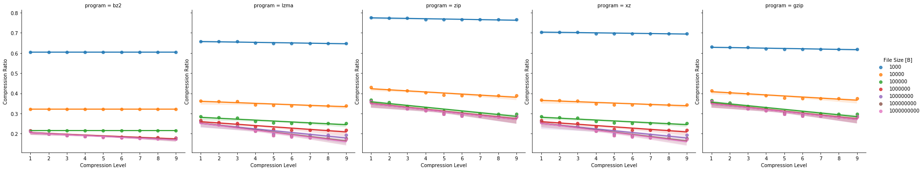
First, let’s check the compression size and time needed. The Compression Ratio of 0.3 means that the compressed file has size of 0.3 of the size of the original file.
ax = sns.lmplot(x="compression_level", y="compression_time", hue="input_file_size", order=1, col="program", data=data, legend=False)
ax.set(xlabel='Compression Level', ylabel='Compression Time [s]')
ax.add_legend(title="File Size [B]")
plt.show()

ax = sns.lmplot(x="compression_level", y="compression_ratio", hue="input_file_size", order=1, col="program", data=data, legend=False)
ax.set(xlabel='Compression Level', ylabel='Compression Ratio')
ax.add_legend(title="File Size [B]")
plt.show()
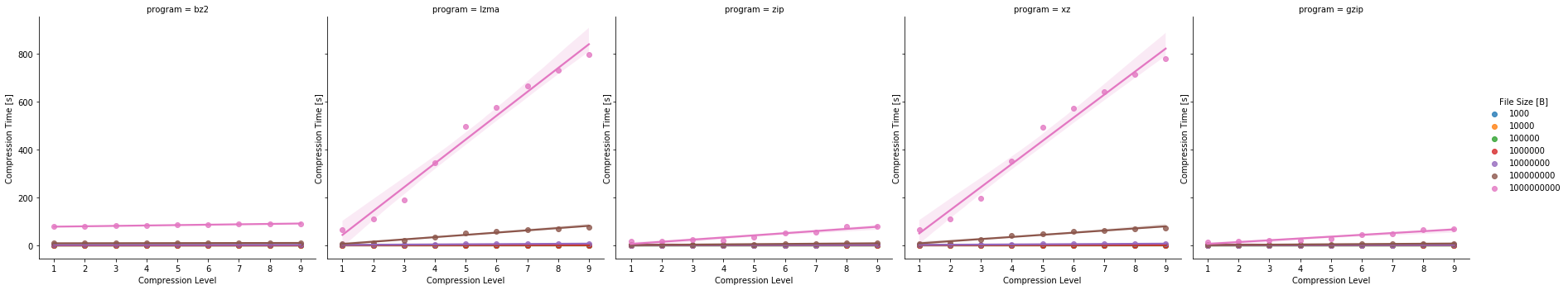
The first thing we can notice is the totally different timing for the lzma and xz programs. The charts look the same, this is mainly because they use the same algorithm.
The best compression ratio was achieved using lzma/xz with compression ratio=9. The only problem was with the compression time, which is rather terrible compared to the bz2 (which has similar ratio but much smaller time).
Also, notice that for the larger files the compression ratio is much better for the larger compression level arguments.
Let’s check the numeric values for the 1GB file for the best compression level:
lzma_info = data[
      (data['compression_level'] == 9)
    & (data['input_file_size'] == 1000000000)
]

lzma_info[['program', 'compression_time', 'decompression_time', 'compression_ratio', 'compression_level']]
.dataframe tbody tr th {
    vertical-align: top;
}

.dataframe thead th {
    text-align: right;
}
As you can see, bzip2 can make the same file size (17% of the original file size) but with 11% of the time of the lzma/xz.
However, the decompression time for bzip2 is 31s, compared to 11s for lzma.
Let’s ignore the lzma/xz from now. The time needed for compression makes these programs totally useless, especially when we can have the same compression ratio with bzip2.
Also, let’s see the characteristic of the 3 biggest files: 10MB, 100MB, and 1GB.
data = data[
      (data['program'].isin(['bz2', 'zip', 'gzip']))
    & (data['input_file_size'] >= 10000000)
]
Let’s take a closer look at the same charts as above:
ax = sns.lmplot(x="compression_level", y="compression_time", hue="input_file_size", order=2, col="program", data=data, legend=False)
ax.set(xlabel='Compression Level', ylabel='Compression Time [s]')
ax.add_legend(title="File Size [B]")
plt.show()

ax = sns.lmplot(x="compression_level", y="decompression_time", hue="input_file_size", order=2, col="program", data=data, legend=False)
ax.set(xlabel='Compression Level', ylabel='Decompression Time [s]')
ax.add_legend(title="File Size [B]")
plt.show()
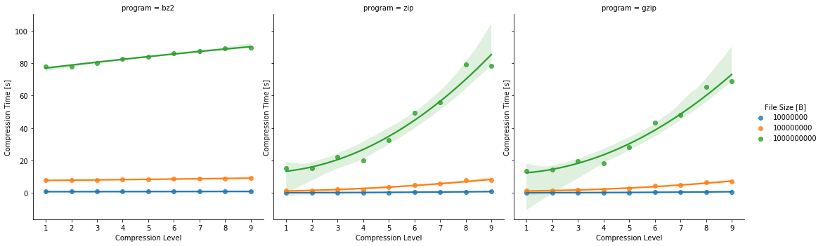
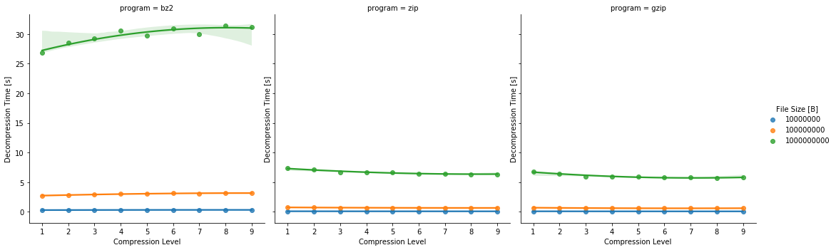
As you can see, the compression time for the Compression Level = 9 for the programs is similar. Let’s stick to this one only:
data = data[(data['compression_level'] == 9)]
Let’s see how fast the files are compressed and decompressed
data = data[[
    "program", "input_file_size_mb", "compression_ratio", "compression_speed",
    "decompression_speed", "compression_time", "decompression_time"]]
data
.dataframe tbody tr th {
    vertical-align: top;
}

.dataframe thead th {
    text-align: right;
}
means=data.groupby('program', as_index=False).mean()
means
.dataframe tbody tr th {
    vertical-align: top;
}

.dataframe thead th {
    text-align: right;
}
Final Remarks
Zip and gzip have similar characteristic, so let’s compare gzip with bzip2.
The bzip2 program makes 40% smaller files. But it’s not for free. The compression time is 30% larger. However, the biggest difference is in the decompression time, bzip2 is 5.4 times bigger.
On the other, hand in case of compressing a 1GB and decompressing the archive, the times are:
| bzip2 | gzip | |
|---|---|---|
| compressing | 89s | 69s |
| decompressing | 31s | 5s |
I think you should answer the question yourself:
is the additional 11% of the archive size worth 5400% longer decompressing time?
lichess_bzip2_size = 267

bz2_compression_ratio = means[means['program']=='bz2']['compression_ratio'].values[0]
print(f"Bzip2 compression ratio {round(bz2_compression_ratio*100)}%")
gzip_compression_ratio = means[means['program']=='gzip']['compression_ratio'].values[0]
print(f"Gzip compression ratio {round(gzip_compression_ratio*100)}%")

unpacked_files_size = lichess_bzip2_size / bz2_compression_ratio
print(f"Estimated size of unpacked files {round(unpacked_files_size)}GB")

lichess_gzip_size = unpacked_files_size * gzip_compression_ratio
print(f"Estimated size of lichess files as compressed with gzip {round(lichess_gzip_size)}GB")

bzip2_decompression_speed = means[means['program']=='bz2'] ['decompression_speed'].values[0]
gzip_decompression_speed  = means[means['program']=='gzip']['decompression_speed'].values[0]

bzip2_decompression_time = (lichess_bzip2_size * 1024) / bzip2_decompression_speed / 3600
gzip_decompression_time  = (lichess_gzip_size * 1024)  / gzip_decompression_speed  / 3600

print(f"Estimated bzip2 decompression time: {round(bzip2_decompression_time)} hours")
print(f"Estimated gzip decompression time: {round(gzip_decompression_time)} hours")
Bzip2 compression ratio 17.0%
Gzip compression ratio 28.0%
Estimated size of unpacked files 1530.0GB
Estimated size of lichess files as compressed with gzip 434.0GB
Estimated bzip2 decompression time: 14.0 hours
Estimated gzip decompression time: 3.0 hours
Small Notes about Chess Files
This analysis is a side effect of my work on analysing lichess data. I have 267GB of bz2 files. With the compression ratio of 17%, the size of the decompressed files is about 1.5TB.
If the files would be packed with gzip, then the archives would have 439GB.
Then the decompressing time would be 3h. In case of the bzip2 files, it’s 14 hours.
As I’m not going to decompress the files, but analyze them using streams (so I will decompress them redirecting the output to an input of a program analyzing the content) it’s possible that I would need to run it more than once.
So, in this case I’m not sure that using bzip2 is a good idea.
Or maybe a good idea would be to repack the bzip2 files to gzip ones.